Machine Learning from Scratch: Linear Regression

Introduction

In this blog post, I’ll be implementing linear regression from scratch in Python. This will be the first in the series of “Machine Learning from Scratch” posts, where I’ll be implementing various machine learning algorithms without using external libraries like scikit-learn, PyTorch or TensorFlow.

I’m doing this in order to understand the underlying concepts of machine learning algorithms and to gain a deeper understanding of how they work under the hood. In the process, I hope to improve my coding skills and learn more about the mathematical concepts behind these algorithms. Additionally, if this helps someone else in their learning journey, that would be great!

Let’s start with a brief overview of Linear Regression.

Linear Regression

Linear regression is a simple machine learning model that is used to predict a continuous target variable based on one or more input features. The model assumes a linear relationship between the input features and the target variable. The goal of linear regression is to find the best-fitting line that minimizes the sum of the squared errors between the predicted and actual values.

Implementation

Let’s move on to the implementation. I’m using numpy for numerical computations and matplotlib for plotting the results. In order to test the model, I’ll be using train_test_split and datasets from scikit-learn to generate some synthetic data.

To implement Linear Regression, I’ll be defining a class LinearRegression with the following methods:

• __init__: Constructor method to initialize the learning rate and number of iterations.
• fit: Method to train the model on the training data.
• predict: Method to make predictions on the test data.

import numpy as np
from sklearn.model_selection import train_test_split
from sklearn import datasets
import matplotlib.pyplot as plt

class LinearRegression:
    def __init__(self, lr=0.001, num_iter=1000):
        self.lr = lr
        self.num_iter = num_iter
        self.weights = None
        self.bias = None

    def fit(self, X, y):
        num_samples, num_features = X.shape
        self.weights = np.zeros(num_features)
        self.bias = 0

        for _ in range(self.num_iter):
            y_pred = np.dot(X, self.weights) + self.bias

            dw = (1/num_samples) * np.dot(X.T, (y_pred - y))
            db = (1/num_samples) * np.sum(y_pred - y)

            self.weights = self.weights - self.lr * dw
            self.bias = self.bias - self.lr * db

    def predict(self, X):
        y_pred = np.dot(X, self.weights) + self.bias
        return y_pred

Now that the class is defined, let’s test it on some synthetic data. We’ll generate some random data using datasets.make_regression and split it into training and testing sets using train_test_split. I’ve also created a helper function rmse to calculate the root mean squared error on the test set.

def rmse(y_test, predictions):
    return np.sqrt(np.mean((y_test - predictions)**2))


if __name__ == '__main__':
    X, y = datasets.make_regression(n_samples=100, n_features=1, noise=20, random_state=42)
    X_train, X_test, y_train, y_test = train_test_split(X, y, test_size=0.2, random_state=42)

    model = LinearRegression(lr=0.01, num_iter=5000)
    model.fit(X_train, y_train)
    predictions = model.predict(X_test)

    error = rmse(y_test, predictions)
    print(f"RMSE: {error}")

    y_pred_line = model.predict(X)
    fig = plt.figure(figsize=(8, 6))
    m1 = plt.scatter(X_train, y_train, s=10)
    m2 = plt.scatter(X_test, y_test, s=10)
    plt.plot(X, y_pred_line, color='black')
    plt.show()

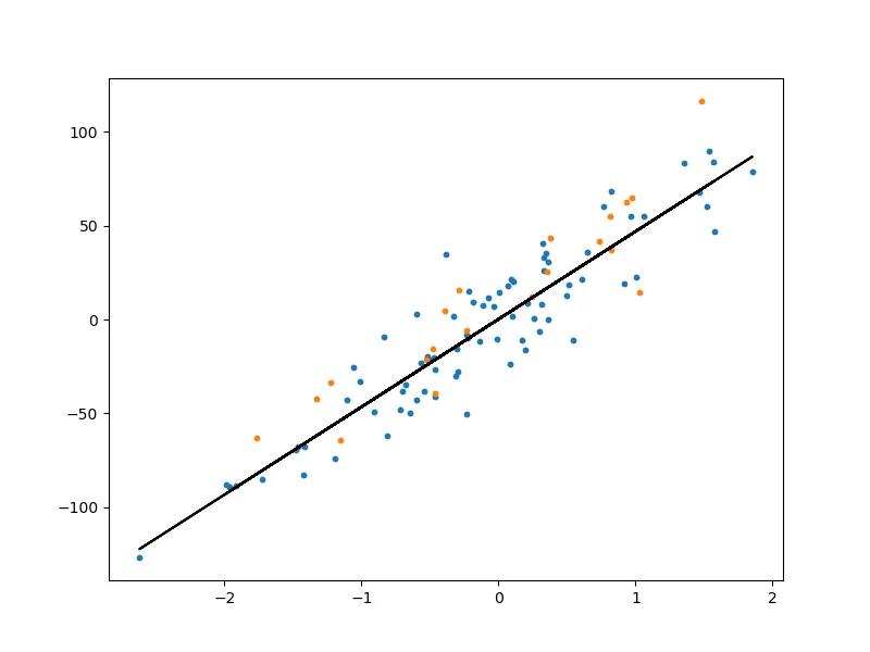
Let’s take a look at the plot to see how well the model is performing:

The model seems to be doing a decent job at predicting the target variable based on the input features.

That’s all for this post. Thanks for reading!